1 Introduction
2 Exploratory Data Analysis
2.1 Categorical variables & booleans
2.1.1 Deeper dive into Cabin
2.1.3 Inferring gender from Name
2.2 Numerical variables
3 Feature Importance
3.1 Mutual information
3.2 Weight of evidence
4 Missing/NAs
4.1 CryoSleep
4.2 Luxury amenities
4.2.1 Cryosleeping individuals
4.2.2 Non-cryosleeping individuals
4.3 HomePlanet
4.4 Deck
4.5 Final roll-up
5 Training
5.1 Splitting into train/validation/test sets
5.2 Random Forest
5.2.1 Fitting process
5.2.2 Validation
5.3 XGBoost
5.3.1 Fitting process
5.3.2 Validation
6 Prediction

1 Introduction

In this report I’ll be tackling the binary classification problem of determining whether a passenger on the Spaceship Titanic has been inadvertently and unfortunately teleported to an alternate dimension. This write-up will be structured in the following general way:

Exploratory data analysis (EDA)
Feature importance using mutual information and weight of information/information value
Imputation and prediction of missing values using the mice package
Model training and validation using random forests
Final prediction for the test set provided by Kaggle

Before we begin, some links and setup code:

This article was originally posted here
This write-up is inspired by the excellent report written by Megan L. Risdal: Exploring Survival on the Titanic
Kaggle competition link

See R libraries used

library(tidyverse)    # Data manipulation and cleaning
library(data.table)   # Same as above & utilities for loading/saving csvs
library(ggplot2)      # Charting
library(scales)       # Prettier printing of values in charts
library(gridExtra)    # Arrange multiple ggplot2 plots on one chart
library(infotheo)     # Mutual information
library(Information)  # Weight of evidence/information value
library(mice)         # Missing value prediction
library(randomForest) # Random forests
library(xgboost)      # XGBoost ML model
library(caret)        # Confusion matrices & grid search
library(ROCR)         # Calculation of AUC and optimal classification thresholds

We can now load the data-sets that Kaggle provides us and then bind them together.

train <- fread('raw-data/train.csv') %>% as_tibble()
test  <- fread('raw-data/test.csv') %>% as_tibble()

all   <- bind_rows(
  train %>% mutate(dataset = 'train'),
  test %>% mutate(dataset = 'test')
)

2 Exploratory Data Analysis

Some quick glimpses at the data to get a sense of what we’re working with:

# We have 15 variables and 12,970 observations
glimpse(all)

## Rows: 12,970
## Columns: 15
## $ PassengerId  <chr> "0001_01", "0002_01", "0003_01", "0003_02", "0004_01", "0…
## $ HomePlanet   <chr> "Europa", "Earth", "Europa", "Europa", "Earth", "Earth", …
## $ CryoSleep    <lgl> FALSE, FALSE, FALSE, FALSE, FALSE, FALSE, FALSE, TRUE, FA…
## $ Cabin        <chr> "B/0/P", "F/0/S", "A/0/S", "A/0/S", "F/1/S", "F/0/P", "F/…
## $ Destination  <chr> "TRAPPIST-1e", "TRAPPIST-1e", "TRAPPIST-1e", "TRAPPIST-1e…
## $ Age          <dbl> 39, 24, 58, 33, 16, 44, 26, 28, 35, 14, 34, 45, 32, 48, 2…
## $ VIP          <lgl> FALSE, FALSE, TRUE, FALSE, FALSE, FALSE, FALSE, FALSE, FA…
## $ RoomService  <dbl> 0, 109, 43, 0, 303, 0, 42, 0, 0, 0, 0, 39, 73, 719, 8, 32…
## $ FoodCourt    <dbl> 0, 9, 3576, 1283, 70, 483, 1539, 0, 785, 0, 0, 7295, 0, 1…
## $ ShoppingMall <dbl> 0, 25, 0, 371, 151, 0, 3, 0, 17, 0, NA, 589, 1123, 65, 12…
## $ Spa          <dbl> 0, 549, 6715, 3329, 565, 291, 0, 0, 216, 0, 0, 110, 0, 0,…
## $ VRDeck       <dbl> 0, 44, 49, 193, 2, 0, 0, NA, 0, 0, 0, 124, 113, 24, 7, 0,…
## $ Name         <chr> "Maham Ofracculy", "Juanna Vines", "Altark Susent", "Sola…
## $ Transported  <lgl> FALSE, TRUE, FALSE, FALSE, TRUE, TRUE, TRUE, TRUE, TRUE, …
## $ dataset      <chr> "train", "train", "train", "train", "train", "train", "tr…

# View cardinality of variables
all %>% 
  select(-dataset) %>% 
  sapply(n_distinct)

##  PassengerId   HomePlanet    CryoSleep        Cabin  Destination          Age 
##        12970            4            3         9826            4           81 
##          VIP  RoomService    FoodCourt ShoppingMall          Spa       VRDeck 
##            3         1579         1954         1368         1680         1643 
##         Name  Transported 
##        12630            3

For completeness, I’ll include the data explanations provided by Kaggle here:

Variable	Description
PassengerId	Unique ID for each passenger, in the format `gggg_pp` where `gggg` represents the travelling group and `pp` is the number of the individual in the group.
HomePlanet	The planet the passenger departed from.
CryoSleep	Whether the passenger chose to be put into cryosleep over the voyage. Passengers in cryosleep are confined to their cabins.
Cabin	The cabin number where the passenger is staying. Takes the form `deck/num/side`, where `side` can be either `P` for Port or `S` for Starboard.
Destination	The planet the individual is travelling to.
Age	The age of the passenger.
VIP	Whether the passenger has paid for special VIP service during the voyage.
RoomService, FoodCourt, ShoppingMall, Spa, VRDeck	Amount the passenger has billed at each of the Spaceship Titanic’s many luxury amenities.
Name	The first and last names of the passenger.
Transported	Whether the passenger was transported to another dimension, the target column.

Already we see some features that are candidates for one form of engineering or another:

PassengerId has travel group information in it
Cabin can be split into deck, room number, and side which may be useful variables

We’ll now split the EDA work into categorical variables and numeric variables.

2.1 Categorical variables & booleans

Let’s first view the distinct value sets and their distributions for the cardinality categorical variables.

ggplot2 code

all %>% 
  # Variables of interest
  select(HomePlanet, Destination, CryoSleep, VIP) %>% 
  gather(variable, value) %>% 
  # Calculating percentage distributions for each value
  group_by(variable, value) %>% 
  summarise(
    n = n(),
    .groups = 'drop'
  ) %>% 
  group_by(variable) %>% 
  mutate(percentage = n / sum(n)) %>% 
  ungroup() %>% 
  # Charting
  ggplot(aes(x = value, y = percentage, label = percent(percentage, accuracy = 0.1))) +
  geom_col() +
  facet_wrap(vars(variable), scales = 'free') +
  # Label formatting
  labs(x = 'Value', y = 'Percent', title = 'Fig 1. Dsn of Categorical Variables') +
  geom_text(
    position = position_dodge(width = .9),
    vjust = -0.5,
    size = 3
  ) + 
  scale_y_continuous(labels = percent)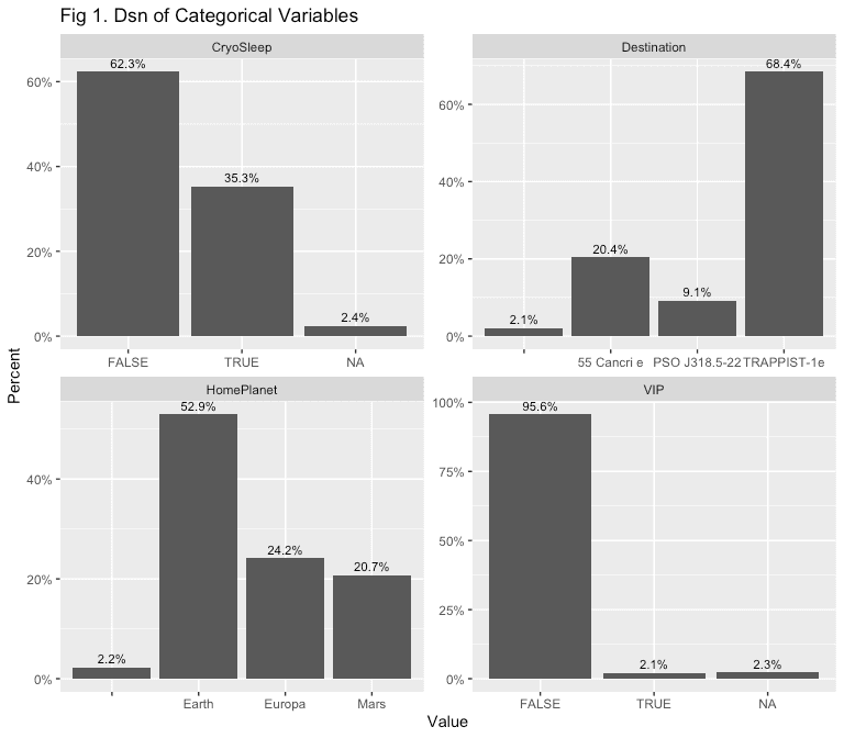

Some takeaways from this chart:

Missing values seem to take the form of empty strings for Destination & HomePlanet;
We’ll want to be careful with the VIP variable since they make up such a small percentage of total passengers;
62.3% of passengers opted to not be put into cryosleep; and,
The majority of passengers have Earth as their home planet, and the majority of passengers are travelling to TRAPPIST-1e.

To round this off, lets use some frequency tables to see how the rate of inadvertent transportation to an alternate dimension varies within each of these variables.

HomePlanet vs. Transported
Destination vs. Transported
CryoSleep vs. Transported
VIP vs. Transported

table(train$HomePlanet, train$Transported) %>% prop.table(1)

##              FALSE      TRUE
##          0.4875622 0.5124378
##   Earth  0.5760539 0.4239461
##   Europa 0.3411544 0.6588456
##   Mars   0.4769756 0.5230244

It appears that people from Europa are transported at a higher frequency, while people from Earth seem to be transported at a lower frequency.

2.1.1 Deeper dive into

Let’s have a closer look at the Cabin variable, and the three substituent pieces of information it provides. First we’ll split the Cabin variable into Deck, Num (room number), and Side, then we’ll view the distributions of the categorical information provided by Deck and Side.

ggplot2 code

all_cabin_spl <- all %>% 
  mutate(Cabin = na_if(Cabin, "")) %>% 
  separate(Cabin, c("Deck", "Num", "Side"), "/")

all_cabin_spl %>% 
  # Variables of interest
  select(Deck, Side) %>% 
  gather(variable, value) %>% 
  # Calculating percentage distributions for each value
  group_by(variable, value) %>% 
  summarise(
    n = n(),
    .groups = 'drop'
  ) %>% 
  group_by(variable) %>% 
  mutate(percentage = n / sum(n)) %>% 
  ungroup() %>% 
  # Charting
  ggplot(aes(x = value, y = percentage, label = percent(percentage, accuracy = 0.1))) +
  geom_col() +
  facet_wrap(vars(variable), scales = 'free') +
  # Label formatting
  labs(x = 'Value', y = 'Percent', title = 'Fig 2. Dsn of Deck and Side') +
  geom_text(
    position = position_dodge(width = .9),
    vjust = -0.5,
    size = 3
  ) + 
  scale_y_continuous(labels = percent)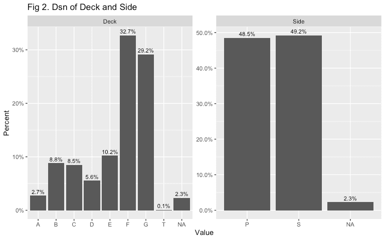

At a glance, passengers tend to be more heavily weighted towards decks F and G, with a very small allocation to deck T. The distribution between port and starboard sides seems to be around equal.

Let’s quickly check how the rate of transportation to an alternative dimension varies with these features:

Deck vs. Transported
Side vs. Transported

# Pull only examples from the training dataset as these have non-NA Transported values
train_cabin_spl <- all_cabin_spl %>% filter(dataset == 'train') %>% select(-dataset)

table(train_cabin_spl$Deck, train_cabin_spl$Transported) %>% prop.table(1)

##         FALSE      TRUE
##   A 0.5039062 0.4960938
##   B 0.2657253 0.7342747
##   C 0.3199465 0.6800535
##   D 0.5669456 0.4330544
##   E 0.6426941 0.3573059
##   F 0.5601288 0.4398712
##   G 0.4837827 0.5162173
##   T 0.8000000 0.2000000

Passengers on decks B, C, E, T all seem to be transported at a varying rate.

2.1.2 Deeper dive into

Let’s see if the traveller’s group size will be helpful for our purposes, first we’ll see what the distribution of group sizes looks like.

Manipulation & ggplot2 code

# Separate the PassengerId variable into a Group and Passenger ID.
all_grp_sep <- all %>% 
  separate(PassengerId, c('GroupId', 'PassengerId'), "_")

# Get number of individuals within each group ID.
all_grps <- all_grp_sep %>% 
  distinct(GroupId, PassengerId) %>% 
  group_by(GroupId) %>% 
  summarise(
    group_size = n(), 
    .groups = 'drop'
  )

# View distribution of group sizes
all_grps %>% 
  ggplot(aes(x = group_size)) +
  geom_histogram(bins = 30) +
  scale_x_continuous(breaks = unique(all_grps$group_size) %>% sort()) +
  scale_y_continuous(labels = comma) +
  labs(x = 'Group Size', y = "Count", title = "Fig 3. Distribution of Travel Group Sizes")

To round this out, we’ll have a quick look at how alternate dimension transportation varies across group sizes.

# Add the new group size variable onto the main dataset then filter only for the training set
all_grouped <- all_grp_sep %>% left_join(all_grps, by = 'GroupId')

train_grouped <- all_grouped %>% filter(dataset == 'train') %>% select(-dataset)

table(train_grouped$group_size, train_grouped$Transported) %>% prop.table(1)

##         FALSE      TRUE
##   1 0.5475546 0.4524454
##   2 0.4619501 0.5380499
##   3 0.4068627 0.5931373
##   4 0.3592233 0.6407767
##   5 0.4075472 0.5924528
##   6 0.3850575 0.6149425
##   7 0.4588745 0.5411255
##   8 0.6057692 0.3942308

It looks like transportation rate varies a little bit with group size.

That’s it for the categorical variables, we’ll move on to the numerical variables now.

2.1.3 Inferring gender from

For this application, we’ll use genderize.io to infer a person’s gender based on their first name. This API works by checking which gender was most likely to be the case for given an input first name over the data they have gathered from across the web. Note there are some caveats to using this approach:

There are some names that this API cannot predict genders for; these people are given a gender of unknown;
The gender of a first name can change based on both the date of birth and location/country context - this has been ignored for now (noting we do not have access to country of origin data here as well);
This is also currently a naive approach that takes the first word of the Name string as the first name of the individual, no considerations have been made for countries that have different name orders (e.g. where family name comes first).

With that being said, to infer genders for the names in the dataset, a unique list of first names is extracted and then ran through genderize’s CSV tool. This was done as opposed to using native libraries that access this API such as genderizeR or GenderGuesser since genderize has a limit of 1000 queries per day and it was just easier to run the names through the provided CSV tool manually.

# Split the name variable into first and last names, then get unique list of names in data-set to run
# through genderize.io 
all_name_split <- all_grouped %>% 
  separate(Name, c("first_name", "last_name"), extra = 'merge', fill = 'right')

all_name_split %>% distinct(first_name) %>% nrow() # 2,884 - 3 days worth of queries

## [1] 2884

Using genderize.io's CSV tool

# Split the distinct list of first names into 3 parts, with max 1,000 rows each
split_name_list <- all_name_split %>% 
  distinct(first_name) %>% 
  split(rep(1:ceiling(nrow(.) / 1000), each = 1000, length.out = nrow(.)))

for (i in 1:length(split_name_list)) {
  fwrite(split_name_list[[i]], paste0('output/intermediate/', i, '.csv'))
}

#### Run through genderize.io's CSV tool

# Check for names that may have been missed by the API
all_name_split %>% 
  distinct(first_name) %>% 
  anti_join(
    bind_rows(
      fread('other-inputs/1_genderize.csv'),
      fread('other-inputs/2_genderize.csv'),
      fread('other-inputs/3_genderize.csv')
    )
    , by = 'first_name'
  ) %>%
  fwrite('output/intermediate/4.csv')

# Check that all names have now been genderised
gender_lookup <- bind_rows(
  fread('other-inputs/1_genderize.csv'),
  fread('other-inputs/2_genderize.csv'),
  fread('other-inputs/3_genderize.csv'),
  fread('other-inputs/4_genderize.csv'),
)

all_name_split %>% 
  distinct(first_name) %>% 
  anti_join(gender_lookup, by = 'first_name') %>%
  nrow() == 0
## [1] TRUE

# Add these back to the main dataset
all_gendered <- all_grouped %>% 
  separate(Name, c("first_name", "last_name"), extra = 'merge', fill = 'right') %>% 
  left_join(gender_lookup, by = 'first_name')

train_gendered <- all_gendered %>% filter(dataset == 'train')

Let’s see quickly if transportation rate tends to vary with gender.

table(train_gendered$gender, train_gendered$Transported) %>% prop.table(1)

##               FALSE      TRUE
##   female  0.5514810 0.4485190
##   male    0.5074228 0.4925772
##   unknown 0.4186420 0.5813580

It looks like male passengers were transported at a slightly higher rate than female passengers.

2.2 Numerical variables

The following are the numeric variables available to us as well as their quartiles and number of NAs present.

# All stock features
all %>% 
  select(-dataset) %>% 
  select_if(is.numeric) %>% 
  summary()

##       Age         RoomService        FoodCourt      ShoppingMall    
##  Min.   : 0.00   Min.   :    0.0   Min.   :    0   Min.   :    0.0  
##  1st Qu.:19.00   1st Qu.:    0.0   1st Qu.:    0   1st Qu.:    0.0  
##  Median :27.00   Median :    0.0   Median :    0   Median :    0.0  
##  Mean   :28.77   Mean   :  222.9   Mean   :  452   Mean   :  174.9  
##  3rd Qu.:38.00   3rd Qu.:   49.0   3rd Qu.:   77   3rd Qu.:   29.0  
##  Max.   :79.00   Max.   :14327.0   Max.   :29813   Max.   :23492.0  
##  NA's   :270     NA's   :263       NA's   :289     NA's   :306      
##       Spa              VRDeck       
##  Min.   :    0.0   Min.   :    0.0  
##  1st Qu.:    0.0   1st Qu.:    0.0  
##  Median :    0.0   Median :    0.0  
##  Mean   :  308.5   Mean   :  306.8  
##  3rd Qu.:   57.0   3rd Qu.:   42.0  
##  Max.   :22408.0   Max.   :24133.0  
##  NA's   :284       NA's   :268

# + the room number of the passenger
all_cabin_spl %>% 
  select(Num) %>% 
  mutate(Num = as.numeric(Num)) %>% 
  summary()

##       Num        
##  Min.   :   0.0  
##  1st Qu.: 170.0  
##  Median : 431.0  
##  Mean   : 603.6  
##  3rd Qu.:1008.0  
##  Max.   :1894.0  
##  NA's   :299

Let’s view the distributions of these variables for those that were transported and those that weren’t to see if we can spot any relationships.

ggplot2 code

train_cabin_spl %>% 
  mutate(Num = as.numeric(Num)) %>% 
  # Select variables that are numeric or those named 'Transported' (the target)
  select_if(sapply(., is.numeric) | str_detect(names(.), "Transported")) %>% 
  gather(variable, value, -Transported) %>% 
  # Charting
  ggplot(aes(x = value, fill = Transported)) +
  geom_histogram(position = 'dodge', bins = 30) +
  # Split charts by variable
  facet_wrap(vars(variable), scales = 'free') +
  # Labels and legends
  scale_y_continuous(labels = comma) +
  scale_x_continuous(labels = comma) +
  theme(legend.position = "bottom") + 
  labs(x = 'Value', y = 'Count', title = 'Fig 4. Dsn of Numeric Variables vs Target ')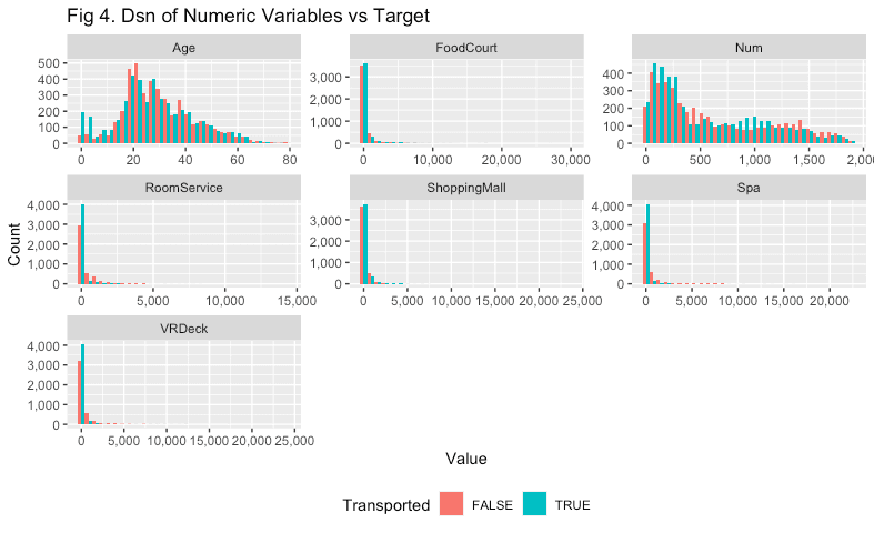

Nothing particularly illuminating here, although it seems like younger children are more likely to be transported than others.

3 Feature Importance

While we’ve developed hypotheses regarding which features may have value in predicting whether an individual has been transported, let’s back these with some formal analysis. We’ll use mutual information to rank the features in terms of relationship with the target variable, then weight of evidence/information value to rank features and determine which features we’ll use in our random forest.

Manipulation code

# Prep the dataset - all_wrk will have both our PassengerId and GroupId variables split out, as well as our group size variable
all_wrk <- all_cabin_spl %>% 
  separate(PassengerId, c('GroupId', 'PassengerId'), "_") %>% 
  left_join(all_grps, by = 'GroupId') %>% 
  mutate_all(.funs = ~ na_if(., "")) %>% 
  separate(Name, c("first_name", "last_name"), extra = 'merge', fill = 'right') %>% 
  left_join(gender_lookup, by = 'first_name')

# We'll pull the training subset of this data-set since we want to compare values to the target
train_wrk <- all_wrk %>% filter(dataset == 'train') %>% select(-dataset)

3.1 Mutual information

Mutual information is the first feature utility metric we’ll use to rank our features and is advantageous since it measures relationships whether they are linear or non-linear. Mutual information essentially measures the extent to which knowledge of one variable reduces uncertainty about another.

We’ll be using the infotheo package to perform this part of the analysis.

Mutual information & ggplot2 code

# Set up a data-frame that tracks variables and their mutual information value which we'll fill in...
mutual_info <- tibble(
  variable = train_wrk %>% select(-Transported, -GroupId, -PassengerId, -Num, -ends_with('_name')) %>% colnames(),
  mutual_info = NA_real_
)

# ... with this for-loop
for (i in 1:nrow(mutual_info)) {

  mutual_info[[i, 2]] <- mutinformation(train_wrk[mutual_info[[i, 1]]], train_wrk$Transported)
  
}

# Now that we have our mutual information values, let's create an ordered factor to ensure our plot has them in descending order
mutual_info_fct_order <- mutual_info %>% arrange(mutual_info) %>% pull(variable)

mutual_info <- mutual_info %>% mutate(variable = factor(variable, levels = mutual_info_fct_order))

# Finally, chart the mutual information values
mutual_info %>% 
  ggplot(aes(x = mutual_info, y = variable)) +
  geom_col() +
  labs(x = 'Mutual Information', y = 'Variable', title = 'Fig 5. Mutual Information of Features')

Some of our potential candidates for features actually have low mutual information! Those would be HomePlanet, Destination, Deck, and Age. It seems that the focus is more on the variables that track passenger spending on the luxury amenities, as well as whether the patient has elected to be in CryoSleep or not (this makes sense, as whether a person spends on amenities or not depends on whether a person has elected to go into cryosleep as we’ll see in the next section).

Now that we have a ranking, let’s see if we can validate these and also determine a cut-off for usefulness using weight of evidence analysis.

3.2 Weight of evidence

Weight of evidence (WOE) allows us to rank feature importance, and also provides a benchmark above which we can say the feature is likely to be useful to any prediction efforts we’ll be making. WOE is calculated across a feature column and the scores then aggregated into a value called an Information Value (IV). In general, an IV that is greater than 0.1 indicates at least medium predictive power, we’ll be using this as our baseline IV cutoff for feature importance. We’ll be using the Information package to perform this part of this analysis.

Weight of evidence code

# To do this, we'll need all character variables as factors and logical variables as numerics
train_woe <- train_wrk %>% 
  select(-GroupId, -PassengerId, -ends_with('_name')) %>% 
  # Convert all character columns to factors
  mutate_if(
    is.character,
    factor
  ) %>% 
  # Force Transported to numeric
  mutate(Transported = as.numeric(Transported))

# Calculate Weight of Evidence over each column, then Information Value
inf_value <- create_infotables(data = train_woe, y = "Transported", bins = 10)$Summary

With the Information Values calculated, let’s then compare the order of variables with those produced by the mutual information analysis:

ggplot2 code

# Using gridExtra to arrange two separate ggplot2 charts
grid.arrange(
  mutual_info %>% 
    ggplot(aes(x = mutual_info, y = variable)) +
    geom_col() +
    labs(x = 'Mutual Information', y = 'Variable', title = 'Fig 6. Mutual Information vs.'),
  inf_value %>% 
    mutate(Variable = factor(Variable, levels = inf_value %>% arrange(IV) %>% pull(Variable))) %>% 
    ggplot(aes(x = IV, y = Variable)) +
    geom_col() +
    labs(x = 'Information Value', y = element_blank(), title = 'Information Value') +
    geom_vline(xintercept = 0.1),
  ncol = 2
)

Generally the two measures agree in terms of ranking feature strength. Keeping to our 0.1 Information Value cutoff, the variables we’ll be using in our model are: CryoSleep, RoomService, Spa, VRDeck, ShoppingMall, FoodCourt, Deck, HomePlanet.

4 Missing/NAs

Now that we know what our data looks like and what features we might like to focus on, we can turn our attention to filling in the holes in our data-set.

# Let's create a working copy of the data-set we have at this point that we can modify at will
all_wrk_tmp <- all_wrk

# First thing we'll do is change all NA gender values to 'unknown' as this is what the genderize.io API 
#  applies when it cannot determine a gender.
all_wrk_tmp <- all_wrk_tmp %>% 
  replace_na(list(gender = 'unknown'))

# Count number of rows with at least one NA in it
all_wrk_tmp[rowSums(is.na(all_wrk_tmp %>% mutate_all(.funs = ~ na_if(., "")))) > 0, ] %>% nrow()

## [1] 6364

It looks like 49.1% of the rows in our data-set have at least one NA in them. A substantial amount - we’ll want to plug as many of these holes as we can.

Where do these missing values reside?

(
  all_wrk_tmp %>% 
    mutate_all(.funs = ~ na_if(., "")) %>% 
    sapply(function(x) sum(is.na(x))) / nrow(all_wrk_tmp)
) %>% 
  as.list() %>% 
  data.frame() %>% 
  gather(variable, missing_pct) %>% 
  arrange(desc(missing_pct))

##        variable missing_pct
## 1   Transported  0.32976099
## 2     CryoSleep  0.02390131
## 3  ShoppingMall  0.02359291
## 4          Deck  0.02305320
## 5           Num  0.02305320
## 6          Side  0.02305320
## 7           VIP  0.02282190
## 8    first_name  0.02266769
## 9     last_name  0.02266769
## 10    FoodCourt  0.02228219
## 11   HomePlanet  0.02220509
## 12          Spa  0.02189668
## 13  Destination  0.02112567
## 14          Age  0.02081727
## 15       VRDeck  0.02066307
## 16  RoomService  0.02027756
## 17      GroupId  0.00000000
## 18  PassengerId  0.00000000
## 19      dataset  0.00000000
## 20   group_size  0.00000000
## 21       gender  0.00000000

We’ll be using two strategies to fill these NAs in here. The first being imputation where we infer what the missing values should be based on relationships we find in the dataset, the second being prediction where we use the mice package to predict missing values using random forests.

For now, we’ll focus on filling in values for features that we know will go into our model and features that are related to those.

4.1

Our first clue is that individuals who are put into cryosleep are confined to their cabin for the trip (I should hope so). This is likely to mean that they would have no need to pay for luxury amenities (i.e., RoomService, FoodCourt, ShoppingMall, Spa, and VRDeck should be 0 for those with CryoSleep == TRUE). Let us confirm that this is true throughout the dataset:

all_cryo_sub <- all_wrk_tmp %>% 
  # Create a variable that sums all luxury spend columns
  mutate(lux_spend = ShoppingMall + VRDeck + FoodCourt + Spa + RoomService)

all_cryo_sub %>% filter(CryoSleep & lux_spend > 0) %>% nrow() == 0

## [1] TRUE

We can now be fairly certain that we can use this relationship to infer that the value of CryoSleep is FALSE when the sum of all luxury spending is greater than 0.

Note that we don’t have the information to infer the converse - i.e. we cannot assume that CryoSleep is TRUE when luxury spending is 0. Someone that committed no money to the spaceship’s luxury amenities may have just not been attracted to the Titanic’s offerings. It would be interesting to test this though, let’s calculate the observed conditional probability that a person chose to be in cryosleep, given that they spent no money on luxury amenities.

(
  nonspender_cryosleep_rate <- all_wrk_tmp %>% 
    mutate(lux_spend_keepnas = ShoppingMall + VRDeck + FoodCourt + Spa + RoomService) %>% 
    filter(!is.na(CryoSleep) & lux_spend_keepnas == 0) %>% 
    group_by(CryoSleep) %>% 
    tally() %>% 
    mutate(pct = n / sum(n)) %>% 
    filter(CryoSleep) %>% 
    pull(pct)
)

## [1] 0.8591341

It’s pretty high! Let’s keep this rate in our back pocket to validate our results once our imputations and predictions are complete for the CryoSleep feature.

For now, let’s put what we’ve learnt into effect and assign FALSEs to CryoSleep where luxury spend is > 0:

Manipulation code

all_wrk_tmp <- all_wrk_tmp %>% 
  mutate(
    # Create a sum of all luxury spends, allowing NAs to flow through so we don't accidentally catch any in the following statement
    lux_spend_ignorenas = rowSums(select(., ShoppingMall, VRDeck, FoodCourt, Spa, RoomService), na.rm = TRUE),
    # Impute the value of CryoSleep where the sum of luxury spend (where all values of luxury spend were available) is non-zero
    CryoSleep = case_when(
      is.na(CryoSleep) & lux_spend_ignorenas > 0 ~ FALSE,
      TRUE ~ CryoSleep
    )
  )

For CryoSleep where luxury spend isn’t greater than zero, we’ll use the mice package to predict missing values with random forests.

Manipulation code

# Create imputation
imput_cryosleep <- all_wrk_tmp %>%
  mutate(
    HomePlanet_fct = factor(HomePlanet), 
    Destination_fct = factor(Destination), 
    Deck_fct = factor(Deck)
  ) %>%
  select(CryoSleep, HomePlanet_fct, Destination_fct, Deck_fct, ShoppingMall, VRDeck, FoodCourt, Spa, RoomService) %>%
  mice(method = 'rf', seed = 24601, maxit = 1) %>% # Who am I?
  complete() %>% 
  mutate(CryoSleep = as.logical(CryoSleep)) %>% 
  select(-ends_with('_fct'))

# Let's quickly check the percentage of passengers who spend 0 on luxury amenities and who were also in cryosleep to compare against what we calculated earlier
imput_cryosleep %>% 
  mutate(lux_spend_keepnas = ShoppingMall + VRDeck + FoodCourt + Spa + RoomService) %>% 
  filter(!is.na(CryoSleep) & lux_spend_keepnas == 0) %>% 
  group_by(CryoSleep) %>% 
  tally() %>% 
  mutate(pct = n / sum(n)) %>% 
  filter(CryoSleep) %>% 
  pull(pct)

Pretty close to our previously calculated rate of 85.9%.

To wrap up for the cryosleep imputation, we’ll add the filled in values back to the main dataset and compare the distribution of imputed values against those that were there originally.

ggplot2 code

all_wrk_tmp <- all_wrk_tmp %>% 
  select(-CryoSleep) %>% 
  bind_cols(imput_cryosleep %>% select(CryoSleep))

# See if imputed values on aggregate change the distribution
all_wrk %>%
  filter(!is.na(CryoSleep)) %>% 
  group_by(CryoSleep) %>% 
  # Get number of rows for CryoSleep == TRUE and CryoSleep == FALSE
  tally() %>% 
  mutate(dataset = 'Unmodified') %>% 
  bind_rows(
    all_wrk_tmp %>% 
      filter(!is.na(CryoSleep)) %>% 
      group_by(CryoSleep) %>% 
      tally() %>% 
      mutate(dataset = 'Imputed')
  ) %>% 
  group_by(dataset) %>% 
  mutate(pct = n / sum(n)) %>% 
  ungroup() %>% 
  # Charting
  ggplot(aes(x = dataset, fill = CryoSleep, y = pct, label = percent(pct, 0.1))) +
  geom_col(position = 'dodge') +
  # Labels and theme
  scale_y_continuous(labels = percent) +
  labs(x = 'Dataset', y = 'Percent', title = 'Fig 7. Imputed vs. original dataset') +
  geom_text(
    position = position_dodge(width = .9),
    vjust = -0.5,
    size = 3
  ) +
  theme(legend.position = 'bottom')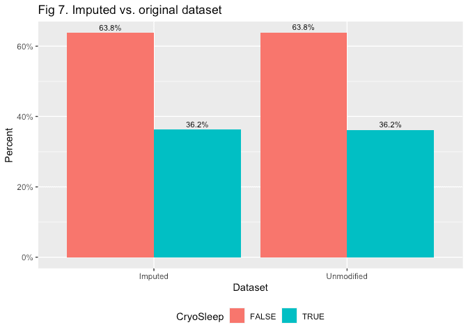

4.2 Luxury amenities

4.2.1 Cryosleeping individuals

Given what we’ve learnt in the previous section, we can infer that the luxury spend for people in cryosleep will be zero.

all_wrk_tmp <- all_wrk_tmp %>% 
  # Where CryoSleep == TRUE and a luxury spend variable is NA, make it 0.
  mutate_at(
    .vars = vars(ShoppingMall, VRDeck, FoodCourt, Spa, RoomService),
    .funs = ~ ifelse(CryoSleep & is.na(.), 0, .)
  )

4.2.2 Non-cryosleeping individuals

Looking through the distributions of other variables vs. luxury spend, there aren’t many convincing relationships we can draw on to impute missing values for individuals who aren’t cryosleeping. However, there are some patterns visible in the data:

ggplot2 code

all_wrk_tmp %>%
  filter(!CryoSleep) %>%
  mutate(lux_spend = ShoppingMall + VRDeck + FoodCourt + Spa + RoomService) %>%
  ggplot(aes(y = lux_spend, x = Destination, fill = HomePlanet)) +
  geom_boxplot() +
  scale_y_continuous(labels = dollar) +
  labs(x = 'Destination', y = 'Total Luxury Spend', title = 'Fig 8a. Luxury spend vs. Destination, Home Planet')

ggplot2 code

all_wrk_tmp %>%
  filter(!CryoSleep) %>%
  mutate(lux_spend = ShoppingMall + VRDeck + FoodCourt + Spa + RoomService) %>%
  mutate(Num = as.numeric(Num)) %>%
  ggplot(aes(x = Num, y = lux_spend, colour = HomePlanet)) +
  geom_point() +
  scale_y_continuous(labels = dollar) +
  scale_x_continuous(labels = comma) +
  labs(x = 'Number', y = element_blank(), title = 'Fig 8b. Luxury spend vs. Room number, Home Planet')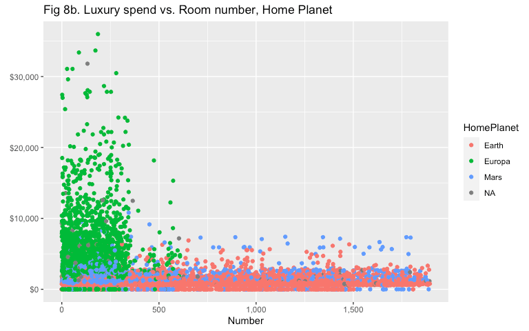

For now, we’ll predict the remaining luxury spend values on some variables such as HomePlanet, Destination, and Deck - variables that seem to have some association with luxury spend.

Manipulation code

# Pull out examples where CryoSleep is not TRUE
all_wrk_noncryo <- all_wrk_tmp %>% filter(!CryoSleep | is.na(CryoSleep))
  
imput_lux_spend <- all_wrk_noncryo %>% 
  mutate(
    HomePlanet_fct = factor(HomePlanet), 
    Destination_fct = factor(Destination), 
    Deck_fct = factor(Deck)
  ) %>% 
  select(HomePlanet_fct, Destination_fct, Deck_fct, ShoppingMall, VRDeck, FoodCourt, Spa, RoomService) %>% 
  mice(method = 'rf', seed = 24601, maxit = 1) %>% 
  complete() %>% 
  select(-ends_with('_fct'))

Finally, we’ll add the predicted values back to the dataset, and compare the distributions of predicted/imputed values vs. the original dataset.

Manipulation and ggplot2 code

all_wrk_tmp <- all_wrk_tmp %>% 
  # Filter out !CryoSleep and is.na(CryoSleep) as they're contained in all_wrk_noncryo
  filter(CryoSleep) %>% 
  bind_rows(
    all_wrk_noncryo %>%
      select(-ShoppingMall, -VRDeck, -FoodCourt, -Spa, -RoomService) %>% 
      bind_cols(
        imput_lux_spend %>% 
          select(ShoppingMall, VRDeck, FoodCourt, Spa, RoomService)
      )
  ) %>% 
  mutate(lux_spend = ShoppingMall + VRDeck + FoodCourt + Spa + RoomService)

all_wrk %>% 
  select(ShoppingMall, VRDeck, FoodCourt, Spa, RoomService) %>% 
  mutate(dataset = 'Unmodified') %>% 
  bind_rows(
    all_wrk_tmp %>% 
      select(ShoppingMall, VRDeck, FoodCourt, Spa, RoomService) %>% 
      mutate(dataset = 'Imputed')
  ) %>% 
  gather(variable, value, -dataset) %>% 
  ggplot(aes(x = value, fill = dataset)) +
  geom_histogram(position = 'dodge') +
  facet_grid(rows = vars(variable), scales = 'free') +
  theme(legend.position = 'bottom') +
  scale_x_continuous(limits = c(NA, 10000), labels = comma) +
  scale_y_continuous(labels = comma) +
  labs(x = 'Value', y = 'Count', fill = 'Dataset', title = 'Fig 9. Imputed vs. original dataset')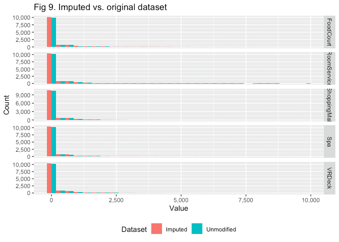

4.3

Looking at the deck of a passenger vs. their home planet, it looks like we can reasonably infer that if you are on decks A, B, C, or T, your HomePlanet was Europa. Further, it looks like deck G is only inhabited by people from Earth.

ggplot2 code

all_wrk_tmp %>% 
  group_by(HomePlanet, Deck) %>% 
  tally() %>% 
  ggplot(aes(x = Deck, y = n, fill = HomePlanet)) +
  geom_col(position = 'dodge') +
  scale_y_continuous(labels = comma) +
  labs(y = 'Count', title = 'Fig 10. HomePlanet vs. Deck')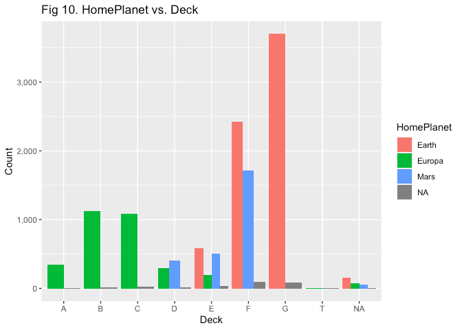

Manipulation code

# Apply this rule to the dataset
all_wrk_tmp <- all_wrk_tmp %>% 
  mutate(
    HomePlanet = case_when(
      is.na(HomePlanet) & Deck %in% c('A', 'B', 'C', 'T') ~ 'Europa',
      is.na(HomePlanet) & Deck == 'G' ~ 'Earth',
      TRUE ~ HomePlanet
    )
  )

We can also hypothesise that people within the same travel group are most likely to have the same home planet. Confirming this:

all_wrk_tmp %>% 
  distinct(GroupId, HomePlanet) %>% 
  filter(!is.na(HomePlanet)) %>% 
  group_by(GroupId) %>% 
  summarise(n = n(), .groups = 'drop') %>% 
  filter(n > 1) %>% nrow() == 0

## [1] TRUE

Manipulation code

# Apply this rule to the dataset
all_wrk_grp_homes <- all_wrk_tmp %>% 
  filter(!is.na(HomePlanet)) %>% 
  distinct(GroupId, HomePlanet) %>% 
  rename(HomePlanet_supplement = HomePlanet)

all_wrk_tmp <- all_wrk_tmp %>% 
  left_join(all_wrk_grp_homes, by = c("GroupId")) %>% 
  mutate(HomePlanet = coalesce(HomePlanet, HomePlanet_supplement), .keep = 'unused')

Finally, we know that there is some association between HomePlanet and room number based on information from the last section, so we’ll use this as one of the values used to predict the remaining NA values:

Manipulation and ggplot2 code

imput_homeplanet <- all_wrk_tmp %>% 
  mutate(
    HomePlanet_fct = factor(HomePlanet),
    Deck_fct = factor(Deck),
    Num_num = as.numeric(Num)
  ) %>% 
  select(HomePlanet_fct, Deck_fct, Num_num) %>% 
  mice(method = 'rf', seed = 24601, maxit = 1) %>% 
  complete() %>% 
  mutate(HomePlanet = as.character(HomePlanet_fct)) %>% 
  select(-ends_with('_fct'), -ends_with('_num'))

# Add these back to the dataset
all_wrk_tmp <- all_wrk_tmp %>% 
  select(-HomePlanet) %>% 
  bind_cols(imput_homeplanet)
  
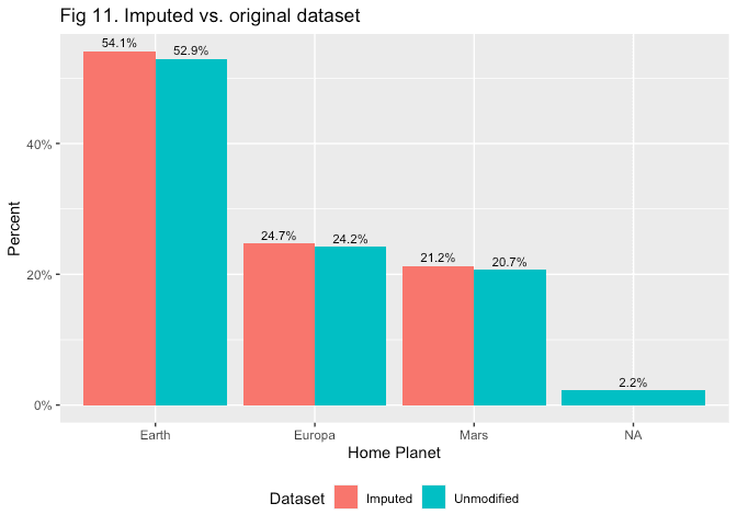
# Check distribution of imputed values
all_wrk %>% 
  group_by(HomePlanet) %>% 
  tally() %>% 
  mutate(pct = n / sum(n)) %>% 
  mutate(dataset = 'Unmodified') %>% 
  bind_rows(
    all_wrk_tmp %>% 
      group_by(HomePlanet) %>% 
      tally() %>% 
      mutate(pct = n / sum(n)) %>% 
      mutate(dataset = 'Imputed')
  ) %>% 
  # Charting
  ggplot(aes(x = HomePlanet, y = pct, fill = dataset, label = percent(pct, 0.1))) +
  geom_col(position = 'dodge') +
  # Labels
  scale_y_continuous(labels = percent) +
  theme(legend.position = 'bottom') +  
  labs(x = 'Home Planet', y = 'Percent', fill = 'Dataset', title = 'Fig 11. Imputed vs. original dataset') +
  geom_text(
    position = position_dodge(width = .9),
    vjust = -0.5,
    size = 3
  )

4.4

There isn’t much to go on for imputing missing Deck values, except for the fact that people within the same travel group tend to stay on decks are in close vicinity to each other.

Manipulation and ggplot2 code

# Get number of people in each group and where they're located
all_wrk_grps <- all_wrk_tmp %>% 
  filter(group_size > 1) %>% 
  select(GroupId, PassengerId, Deck, Num, Side) %>% 
  group_by(GroupId) %>% 
  mutate(count = n()) %>% 
  ungroup() %>% 
  arrange(GroupId, PassengerId)

# Convert the Deck variable to a numeric mapping so that deck distance may be calculated easily
deck_refactor <- tibble(
  Deck = all_wrk_grps %>% filter(!is.na(Deck)) %>% distinct(Deck) %>% pull(Deck) %>% sort(),
  DeckNum = c(1:(all_wrk_grps %>% filter(!is.na(Deck)) %>% distinct(Deck) %>% pull(Deck) %>% length()))
)

all_wrk_grps %>% 
  left_join(deck_refactor, by = 'Deck') %>% 
  group_by(GroupId) %>% 
  summarise(
    range = max(DeckNum) - min(DeckNum),
    .groups = 'drop'
  ) %>% 
  ggplot(aes(x = range)) +
  geom_histogram() +
  scale_y_continuous(labels = comma) +
  labs(x = 'Deck Distance with Groups', y = 'Count', title = 'Fig 12. Dsn of deck distance within groups')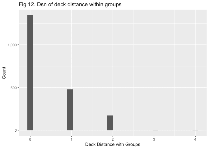

This might enable some sort of modelling of missing deck information based on the deck of others within the group in future, however we’ll go with a simpler method here. Predicting deck with mice doesn’t tend to preserve the distribution we see in the previous chart, so we’ll simply assign missing deck values to a ‘missing’ bucket for now.

all_wrk_tmp <- all_wrk_tmp %>% 
  mutate(Deck = ifelse(is.na(Deck), 'NA', Deck))

4.5 Final roll-up

We’ll do some final checks over the dataset here before we move on to the train/validation/test split and fitting the model.

First, check if there were any missing values we missed in our variables of interest:

all_wrk_tmp %>% 
  select_at(vars(inf_value %>% filter(IV > 0.1) %>% .$Variable)) %>% 
  sapply(function(x) sum(is.na(x)))

##    CryoSleep  RoomService          Spa       VRDeck ShoppingMall    FoodCourt 
##            0            0            0            0            0            0 
##         Deck   HomePlanet 
##            0            0

Let’s impute the value of age in case we need to use it later:

Imputation code

imput_age <- all_wrk_tmp %>% 
  select(-GroupId, -PassengerId, -Transported, -dataset, -Num, -ends_with('_name')) %>% 
  # Convert all character columns to factors
  mutate_if(
    is.character,
    factor
  ) %>%
  mice(method = 'rf', seed = 24601, maxit = 1) %>% 
  complete()

all_wrk_tmp <- all_wrk_tmp %>% 
  select(-Age) %>% 
  bind_cols(imput_age %>% select(Age))

Next, we’ll check that we haven’t lost any people during this process:

identical(
  all_wrk %>% distinct(GroupId, PassengerId) %>% arrange_all(),
  all_wrk_tmp %>% distinct(GroupId, PassengerId) %>% arrange_all()
)

## [1] TRUE

Finally, we’ll convert all character and logical/boolean features into factors for our random forest model.

Manipulation code

all_wrk_final <- all_wrk_tmp %>% 
  mutate_at(
    .vars = vars(Transported, CryoSleep, Deck, HomePlanet),
    .funs = factor
  )

5 Training

5.1 Splitting into train/validation/test sets

We’ll split the dataset back into it’s original train and test groupings, then split the training set down further into a training set and a validation set with a 70%/30% split.

test_clean <- all_wrk_final %>% filter(dataset == 'test') %>% select(-dataset)
train_clean <- all_wrk_final %>% filter(dataset == 'train') %>% select(-dataset)

We’ll be a little careful when splitting the training set into a train/validation set. We do not want people from the same group to be spread across the two sets - this likely has the potential to cause target leakage.

First lets check that there are no groups that are split up between the provided train and test sets:

all_wrk_final %>% 
  distinct(GroupId, dataset) %>% 
  group_by(GroupId) %>% 
  tally() %>% 
  ungroup() %>% 
  filter(n > 1) %>% 
  nrow() == 0

## [1] TRUE

Next, how we’ll do this is we’ll split on distinct GroupId as opposed to randomly sampling 70%/30% of train_clean’s rows. This will not net us an exact 70%/30% split, but it will be good enough for our purposes.

set.seed(24601)
training_proportion <- 0.7

train_val_split <- train_clean %>% 
  group_by(GroupId) %>% 
  # Get count of rows under each GroupId
  tally() %>% 
  # Generate a random number for each row which will be compared against the 
  #  probability of being in the test set (70%).
  mutate(rand = runif(nrow(.))) %>% 
  mutate(grouping = ifelse(rand < training_proportion, 'train', 'validation'), .keep = 'unused')

# Confirm this preserves the ~70/30 split for the most part:
train_val_split %>% 
  group_by(grouping) %>% 
  summarise(n = sum(n), .groups = 'drop') %>% 
  mutate(pct = percent(n / sum(n), 0.1))

## # A tibble: 2 × 3
##   grouping       n pct  
##   <chr>      <int> <chr>
## 1 train       6100 70.2%
## 2 validation  2593 29.8%

# Split train_clean based on the decided GroupId arrangement
train_new <- train_clean %>% filter(GroupId %in% (train_val_split %>% filter(grouping == 'train') %>% .$GroupId))
valid_new <- train_clean %>% filter(GroupId %in% (train_val_split %>% filter(grouping == 'validation') %>% .$GroupId))

5.2 Random Forest

5.2.1 Fitting process

We’ll input our training set into the random forest model now, then plot the out-of-bag (OOB) error across each iteration. A random forest is an ensemble model consisting of a number of decision trees trained on a random subset (Drawn with replacement) of the available training data. Out-of-bag error simply measures the error of the model on the subset of training data that wasn’t used in a given decision tree.

set.seed(24601)

# As a reminder, here's a list of our features of interest
( features_of_interest <- c(inf_value %>% filter(IV > 0.1) %>% .$Variable, 'Age', 'gender') %>% paste(collapse = " + ") )

## [1] "CryoSleep + RoomService + Spa + VRDeck + ShoppingMall + FoodCourt + Deck + HomePlanet + Age + gender"

Random forest training

st_rf_mod <- randomForest(
  as.formula(
    paste('Transported', "~", features_of_interest)
  ),
  data = train_new
)

# Plot OOB error
plot(st_rf_mod, main = 'Fig 13. Random Forest OOB Error')
legend(
  'topright',
  colnames(st_rf_mod$err.rate),
  col = 1:3,
  fill = 1:3
)

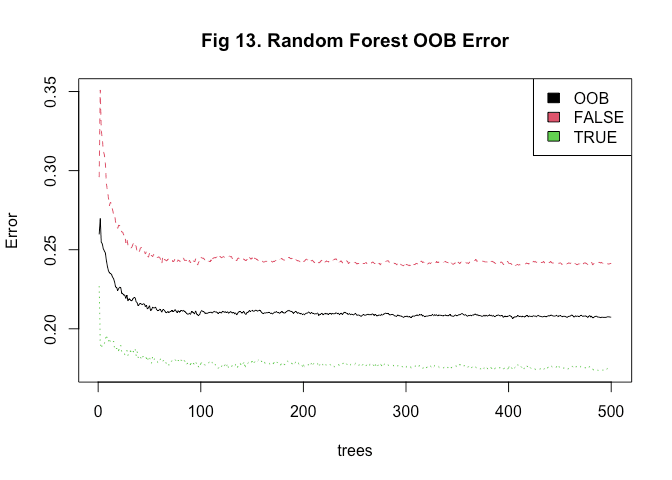
We can see that at the end of the fitting process, the model has an OOB error of 0.207377. The red and green lines show the error in predicting whether a person was not transported and whether a person was transported respectively; with the error in predicting whether a person was transported generally being lower (0.1743772 vs 0.2412762).

We’ll take a quick look at variable importance before moving on to checking performance over our validation set.

Variable importance

# Plot variable importance
importance_output <- importance(st_rf_mod)
importance <- tibble(
  var = row.names(importance_output), 
  imp = round(importance_output[ ,'MeanDecreaseGini'],2)
)

importance %>% 
  mutate(var = factor(var, levels = importance %>% arrange(imp) %>% .$var)) %>% 
  ggplot(aes(x = imp, y = var)) +
  geom_col() +
  labs(x = 'Importance', y = 'Variable', title = 'Fig 14. Random Forest - Variable Importance')

Feature importance generally agrees with the feature utility metrics used previously that Deck and HomePlanet are less important in predicting whether someone was inadvertently teleported or not. The top 6 features in terms of importance are the same top six that appear using mutual information and information value, albeit reshuffled a little bit.

Let’s check the Area under the Curve (AUC) for this model, which can be interpreted as the probability that the model ranks a randomly drawn positive example (i.e. TRUE) correctly before a randomly drawn negative (FALSE). An AUC of 0.5 suggests that the model is no better than a model that randomly classifies the examples it comes across, whereas an AUC of 1.0 suggests that the model is a perfect classifier.

performance(
  prediction(
    predict(st_rf_mod, type = "prob")[,2], 
    as.numeric(train_new$Transported) - 1
  ),
  measure = "auc"
)@y.values[[1]]

## [1] 0.8586274

The Receiver Operating Curve from which the Area under the Curve is derived can also provide us with the optimal cutoff for use as a threshold when classifying examples.

st_rf_cutoff_obj <- performance(
  prediction(
    predict(st_rf_mod, type = "prob")[,2], 
    as.numeric(train_new$Transported) - 1
  ), 
  measure = "cost"
)

( st_rf_optimal_cutoff <- st_rf_cutoff_obj@x.values[[1]][which.min(st_rf_cutoff_obj@y.values[[1]])][[1]] ) 

## [1] 0.5284974

5.2.2 Validation

We’ll now use this model to predict over our validation set, then we’ll check performance metrics such as accuracy, sensitivity, and specificity. Note that, in this case, sensitivity is the ability of the model to correctly identify people who have been transported, and specificity which is the ability of the model to correctly identify someone who has not been transported.

# Predict values and bind to the validation data-frame
predicted_values <- valid_new %>% 
  bind_cols(
    Prediction_prob = predict(st_rf_mod, valid_new, type = 'prob')[,2]
  ) %>% 
  mutate(
    # Utilising the optimal cutoff derived earlier:
    Prediction = ifelse(Prediction_prob > st_rf_optimal_cutoff, TRUE, FALSE),
    Prediction = as.factor(Prediction),
    .keep = 'unused'
  )

# Confusion matrix and accuracy metrics
prediction_cm <- confusionMatrix(
  predicted_values$Prediction, predicted_values$Transported
)

prediction_cm$table

##           Reference
## Prediction FALSE TRUE
##      FALSE   992  205
##      TRUE    314 1082

prediction_cm$overall[['Accuracy']]

## [1] 0.7998457

prediction_cm$byClass[['Sensitivity']]

## [1] 0.7595712

prediction_cm$byClass[['Specificity']]

## [1] 0.8407148

Accuracy, sensitivity, and specificity all look okay here, but it should be noted these do not provide the whole picture. Accuracy in particular can be quite misleading when there are substantial class imbalances in the underlying dataset such as when modelling rare events like the prevalence of rare diseases. The sensitivity and specificity measures aim to ameliorate this issue. AUC also tends to be more holistic, assessing the model across all possible classification thresholds.

Before using this model to predict over the test set, let’s take a look at the VIP sub-group. Since they make up a small portion of total passengers, we aren’t expecting the model to have predicted their transportation rate with as much accuracy as the rest of the passengers.

# Confusion matrix for VIP members
prediction_vip_cm <- confusionMatrix(
  (predicted_values %>% filter(VIP))$Prediction, (predicted_values %>% filter(VIP))$Transported
)

prediction_vip_cm$table

##           Reference
## Prediction FALSE TRUE
##      FALSE    36    4
##      TRUE      1   14

prediction_vip_cm$overall[['Accuracy']]

## [1] 0.9090909

prediction_vip_cm$byClass[['Sensitivity']]

## [1] 0.972973

prediction_vip_cm$byClass[['Specificity']]

## [1] 0.7777778

It’s not too bad. Note the sensitivity is greater than that of the aggregate dataset, but the specificity is lower. i.e. We’re more likely to correctly predict that an individual has been transported to an alternate dimension than in the aggregate dataset, but less likely to correctly predict that an individual was not transported to an alternative dimension.

By now we’ve established a good baseline; let’s see if we can improve on this with other models.

5.3 XGBoost

Let’s try using an extreme gradient boosting (XGBoost) model to predict transportation here. XGBoost in an ensemble technique where a single weak classifier is progressively turned into a stronger one by iteratively predicting the residuals from each new model iteration. This approach is understood to control both bias and variance, in contrast to the random forest algorithm which utilises multiple separate models and bootstrapped aggregation (bagging) which mainly controls for high variance in the model.

XGBoost only works over numeric variables, so we’ll need to one-hot encode our factors, we’ll use caret to do this:

XGBoost prep

# Define a function pipeline to clean all three data-frames
xgb_prep <- function(data, iv_threshold = 0.1) {
  
  # Bin Age and filter only for variables we're interested in
  data_tmp <- data %>% 
    mutate(AgeGrp = cut(Age, breaks = 10 * c(-1:10))) %>% 
    select_at(vars(inf_value %>% filter(IV > iv_threshold) %>% .$Variable, AgeGrp, Transported, gender))
  
  # Force logical to numeric
  data_tmp <- data_tmp %>% 
    mutate_at(
      .vars = vars(CryoSleep),
      .funs = ~ as.numeric(.) - 1
    ) %>% 
    # Label needs to be a factor to show this is a classification problem
    mutate(Transported = as.factor(Transported)) 
  
  # One-hot encode Deck and HomePlanet
  dummy_var_model <- dummyVars(~ Deck + HomePlanet + AgeGrp + gender, data = data_tmp)
  
  # Add back to main dataset
  data_tmp <- data_tmp %>% 
    select(-Deck, -HomePlanet, -AgeGrp, -gender) %>% 
    bind_cols(
      predict(dummy_var_model, newdata = data_tmp)
    )
  
  return(data_tmp)
  
}

train_xgb <- xgb_prep(train_new)
valid_xgb <- xgb_prep(valid_new)
test_xgb <- xgb_prep(test_clean)

5.3.1 Fitting process

XGBoost is engineered for fast implementation, so we can experiment with hyperparameters a little easier. Let’s use a method for finding optimal hyperparameters that tends towards the more exhaustive side of things: the grid search. We’ll pass vectors of possible values for each hyperparameter to the train function from the caret package. This will in turn train an XGBoost model across all possible permutations of these possible values, and will then select the model with the lowest Root Mean Squared Error (RMSE).

XGBoost training

# First, define the controls we want to train with; we're choosing 10-fold cross-validation and a grid search
xgb_control <- trainControl(
  method = "cv", 
  number = 5, 
  search = "grid"
)

# Next, listing the possible hyper-parameters we'll train over
#  For hyper-parameters not listed here, we'll use the default value
xgb_hyp_params <- expand.grid(
  max_depth = c(3, 4, 5, 6), # Controls the max depth of each tree; higher values = more chance of over-fitting 
  nrounds = c(1:15) * 50, # Number of trees to go through
  eta = c(0.01, 0.1, 0.2), # Analogous to learning rate
  gamma = c(0, 0.01, 0.1), # The minimum loss reduction required to split the next node
  
  # Default values for remaining hyper-parameters
  subsample = c(0.5, 0.75, 1),
  min_child_weight = 1,
  colsample_bytree = 0.6
)

# Unregister any parallel workers
env <- foreach:::.foreachGlobals
rm(list=ls(name=env), pos=env)

set.seed(24601)

# Training the model
st_xgb_mod <- train(
  Transported ~ ., 
  data = train_xgb, 
  method = "xgbTree", 
  trControl = xgb_control, 
  tuneGrid = xgb_hyp_params
)

Taking a quick look at feature importance, everything seems to generally align with what we’ve seen previously.

Variable importance plot

xgb.plot.importance(
  xgb.importance(
    colnames(train_xgb %>% select(-Transported)), 
    model = st_xgb_mod$finalModel
  )
)
title('Fig 15. XGBoost Feature Importance')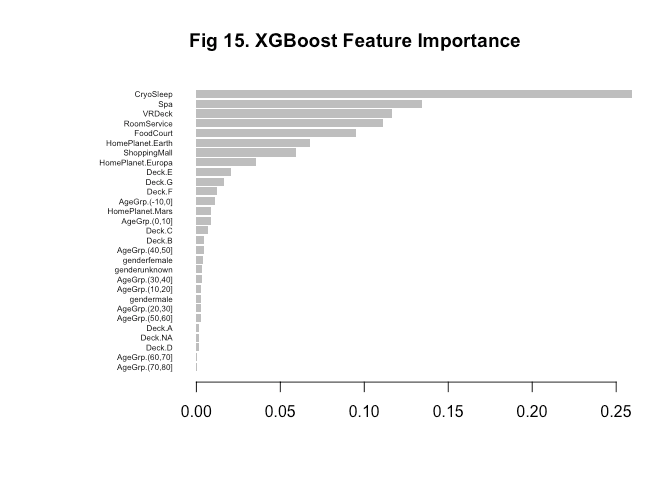

Finally - before we go on to validation, let’s check the AUC and find the optimal classification threshold for this model.

# AUC
performance(
  prediction(
    predict(st_xgb_mod, train_xgb, type = "prob")[,2], 
    as.numeric(train_new$Transported) - 1
  ),
  measure = "auc"
)@y.values[[1]]

## [1] 0.911246

# Optimal cut-off
st_xgb_cutoff_obj <- performance(
  prediction(
    predict(st_xgb_mod, train_xgb, type = "prob")[,2], 
    as.numeric(train_xgb$Transported) - 1
  ), 
  measure = "cost"
)

( st_xgb_optimal_cutoff <- st_xgb_cutoff_obj@x.values[[1]][which.min(st_xgb_cutoff_obj@y.values[[1]])][[1]] )

## [1] 0.5083346

5.3.2 Validation

In validating this model, we see that its done a little better than the random forest we set up earlier. Accuracy, sensitivity, and specificity are all slightly higher than that of the random forest model.

predicted_values_xgb <- valid_new %>% 
  bind_cols(
    Prediction_prob = predict(st_xgb_mod, valid_xgb, type = 'prob')[,2]
  ) %>% 
  mutate(
    Prediction = ifelse(Prediction_prob > st_xgb_optimal_cutoff, TRUE, FALSE),
    Prediction = as.factor(Prediction),
    .keep = 'unused'
  )

# Confusion matrix and accuracy metrics
prediction_cm_xgb <- confusionMatrix(
  predicted_values_xgb$Prediction, predicted_values_xgb$Transported
)

prediction_cm_xgb$table

##           Reference
## Prediction FALSE TRUE
##      FALSE   998  199
##      TRUE    308 1088

prediction_cm_xgb$overall[['Accuracy']]

## [1] 0.8044736

prediction_cm_xgb$byClass[['Sensitivity']]

## [1] 0.7641654

prediction_cm_xgb$byClass[['Specificity']]

## [1] 0.8453768

6 Prediction

Finally, let’s use this model to predict over the test set that Kaggle provided.

final_output <- test_clean %>% 
  unite('PassengerId', GroupId:PassengerId, sep = "_") %>% 
  select(PassengerId) %>% 
  bind_cols(
    Transported_prob = predict(st_rf_mod, test_clean, type = 'prob')[,2]
  ) %>% 
  mutate(
    Transported = ifelse(Transported_prob > st_rf_optimal_cutoff, TRUE, FALSE),
    Transported_fct = as.factor(Transported),
    .keep = 'unused'
  ) %>% 
  mutate(Transported = ifelse(Transported_fct == 'TRUE', 'True', 'False'), .keep = 'unused')

nrow(final_output) == 4277 # Size Kaggle expects for this solution

## [1] TRUE

# Write to a csv
# fwrite(final_output, 'output/spaceship_titanic_rf_solution.csv') # Score: 0.79378

final_output_xgb <- test_clean %>% 
  unite('PassengerId', GroupId:PassengerId, sep = "_") %>% 
  select(PassengerId) %>% 
  bind_cols(
    Transported_prob = predict(st_xgb_mod, test_xgb, type = 'prob')[,2]
  ) %>% 
  mutate(
    Transported = ifelse(Transported_prob > st_xgb_optimal_cutoff, TRUE, FALSE),
    Transported_fct = as.factor(Transported),
    .keep = 'unused'
  ) %>% 
  mutate(Transported = ifelse(Transported_fct == 'TRUE', 'True', 'False'), .keep = 'unused')

nrow(final_output_xgb) == 4277

 ## [1] TRUE

# fwrite(final_output_xgb, 'output/spaceship_titanic_rf_solution_xgb.csv') # Score: 0.79588